
Introduction
Feature engineering is a step toward making the data more feasible for various machine learning techniques and, in turn, creating a model that can make more accurate predictions. This data consists of these features, which essentially undergo the feature engineering algorithms. These features can be categorized into two types: continuous and categorical. What does each represent? Let us discuss.
Learn more about AI Services
Types of Features
Continuous features are those that are numerically represented by default. A feature being represented in integer or float could be an indicator that It is a continuous variable. Even though it can be otherwise, such cases are far and in between.
Categorical features on the other hand are those that consists of categorical data. Unlike continuous features, these do not necessarily hold numerical significance and often represent a feature belonging to a certain category.
There are generic algorithms that can be implemented regardless of the nature of the feature and then, there are those that are unique to each data type. We will discuss them as we go along. So now without further ado let us dive into them.
Feature Engineering Techniques
The techniques that we will be discussing today are as follows:
Data Cleaning
Data cleaning may appear to be a mundane and inconsequential step of the process, but it can be the most crucial step. Cleansed data leads to outstanding results using even simpler models. ls. Carelessly cleaned data leads to a “garbage in garbage out” situation.
Before that data can be utilized for any purpose, we need to take the raw, crude and rather morbid data – from a data scientist’s perspective – and convert it to a more cohesive and streamlined form. Quite often the data is missing the values, or the values are quite scattered.
Missing Data
Missing values can be a result of human error or a machine-induced induced error. There is no one absolute way to handle these missing values, but a better understanding of the nature of the missing values and a deeper insight into why they are missing can give us a better intuition of what solution may bring forth the best results.
Types Of Missing Data
The missing values can be categorized into four types:
Structurally Missing Data
Structurally missing data is the data whose absence can be explained using logical reasoning. This means that the absence of the data is not a fault, in fact the presence could be a concern. The absence of ‘yearly earning’ for an infant in a population consensus explains the whole concept quite well.
Missing Completely at Random
Missing completely at random is the data from which no logic or a pattern can be extracted and is completely random. We can distinguish it from the other type by predicting when the values are missing. This is the easiest to deal with because an imputation with any possible value would suffice to fix this, since the premise is that every missing value is random and shares no correlation. In real life, non-existent co-relations are rarely encountered. If methods like regression can predict which instances will have missing values; we can safely assume that this is not MCAR. A more formal technique to test this assumption is Little’s MCAR test.
Missing at Random
In contrast to what the name suggests, Missing at Random refers to data that can be predicted, based on other values in the instance. This assumption is safer in comparison to the MCAR assumption and can be used to curate a solution for the missing values. This missing data of this type can be solved using a predictive algorithm by using more complex statistical imputation.
Missing Not at Random
Missing Not at Random is the most notorious of all data types. This refers to the data that is missing due to a logical reason and requires imputation. Despite all this insight, imputation cannot be effectively performed.
Handling Missing Data
Removal of data
A simple and straightforward solution to the missing value could be to remove such instances. This may even be a suitable solution if the data does not have a lot of missing values. Well, what if they are not? What if there a quite a few missing values? Even in such cases, data removal can be helpful. If the missing values are highly concentrated in one column (more than 70% of the values are missing in a column), removal of that entire column could be an option given that the value is not structurally missing.
In any case other than these, blindly removing data will most definitely lead to the introduction of a bias, as removal will lead to loss of potentially significant data.
Imputation of data
Removing data seems like a simpler option and can be a possible solution in some cases, but as discussed, the data integrity may take a toll. In contrast, data imputation can manifest better results. For imputation, we first need to define, what type of data it is – continuous or categorical – and proceed accordingly.
Continuous Data vs. Categorical Data
Continuous data refers to data that is numerical in nature and holds numerical significance. Variables such as temperature, area, or TIME could fall into this category. Categorical data, in contrast to this, holds numerical (does not hold numerical significance) and non-numerical data. Variables such as color, sex, or age–group.
So, the data can be handled using the following methodologies:
Mean/Median Imputation
This imputation refers to replacing the missing values with the mean or median of the feature. Median replacement works well for the categorical variables as well.
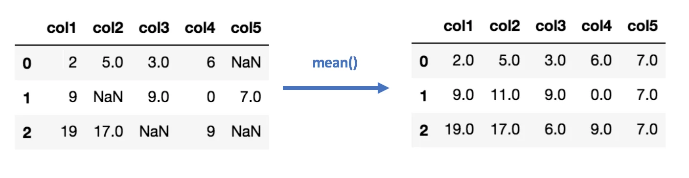
Figure 1: Example of mean imputation
Even though it is quite a simple method and gets the task done, it is not exactly the best solution. The shortcomings of the imputation of this sort are:
- It does not factor in the correlation of the variables.
- It is not an accurate representation of real data
K Nearest Neighbor Imputation
K-nearest neighbor is a classification algorithm that groups the instances in a dataset based on their similarity. KNN-imputation refers to grouping the instances and using the median/mean of the group to input the missing data. This method helps avoid the pitfalls of the simple mean/median imputation as it is a far more accurate representation of the original data, but nothing comes without its vices. The shortcomings of this sort of imputation are:
- It is compute-intensive
- It is prone to outliers
Highlighting Missing Values:
Removing missing values is not the best solution and imputation may not be the best solution either, especially given that the values are structurally missing. Data-Science experts have two different opinions about the efficiency of imputation and argue that if the data is not real, it inherently induces a bias.
Another option can be to mark the values as missing for the model to recognize them as such. For example, in a dataset of a bank’s customer, the variable for loan history could be missing because the customer has never taken a loan. In such cases, we can fill up the values using static values that represent missing data and the machine learning algorithm will recognize the pattern.
Outlier Removal
An outlier refers to a value that does not conform to the prevalent pattern present in the data. A value that is rare and distinct can be considered to be an outlier. An outlier can be a real outlier, or it can be induced by a human or a machine error. Even though it is quite difficult to pinpoint the source of the outlier we can deal with them using methods such as:
Standard Deviation Method
Standard Deviation is the measure to represent the variability of the data with respect to the mean. The following figure represents a dataset and how the data variates from the mean with each standard deviation.
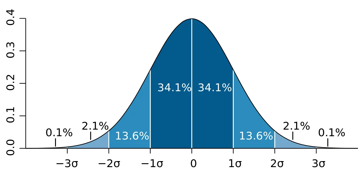
Figure 2: Graphical representation of normal distribution
This measure can be used to remove the outlier. If a value is more than ‘3 standard deviations’ away from the mean, it can be considered an outlier and removed from the dataset. For this to work, a distribution must closely follow the normal distribution otherwise standard deviation measure will not be an accurate representation of the variability of the data.
Inter-Quartile Range Method
Inter Quartile Range is a measure of variability of data, in cases where the data does not follow a Normal Distribution. For the data is divided into four quarters with median being the center of the dataset. The inter-quartile range is demonstrated by ‘Q3-Q1’.
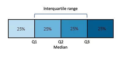
Figure 3: Graphical representation of data distribution in Quartiles
Using this, an outlier can be any value that is greater than (Q3 + 1.5 * IQR) and lesser than (Q1 – 1.5 * IQR).
Empower Your Business with Data Engineering Solutions
Conclusion
So, in this blog, we discussed the data cleaning process in a bigger feature engineering chain. One cannot stress enough in depicting the importance of data cleansing. I will give you some time to wrap your head around these and try to reflect on them in some examples. We will continue with the rest of the processes in the feature engineering chain in my upcoming article.
Stay tuned.