
Introduction
In my previous blog, titled “Feature Engineering Process: A comprehensive guide Part A” I discussed the initial and most crucial step of feature engineering i.e., data cleaning. If you have not read it yet, I would suggest that you read it first for a better understanding of the second part.
FEATURE ENGINEERING PROCESS – PART A
Anyhow! Without further ado, let us dive right back and start with the next phase of feature engineering, the process of ‘Feature Selection’.
Feature Selection
“Not all features are created equal.”
This cannot be any truer. Real life is unfair and so is real-life data, and we must deal with what we are dealt with. Quite often, we are given multitudes of features and not all of them are going to be relevant. It is a data scientist’s job to weed out the useless features.
The question arises that how would we know which is a useless feature?
Let me answer that for you. A useful feature is the one that has some correlation with the predicted variable. For feature selection, we use the Univariate and Bivariate Analysis.
Univariate Analysis
In univariate analysis we try to see if a feature reflects any correlation with the predicted variable. The following figure shows a feature that could be selected using univariate analysis.
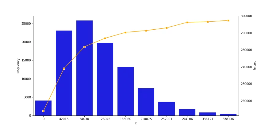
Figure 4: A graph for univariate analysis that shows a strong correlation
Here we can see different graphs that have a correlation with the predicted variable, be it positive or negative. This means that its presence in the feature set will improve the efficacy of the predictions. On the contrary, the following figure represents a very weak co-relation, and such features should be discarded.
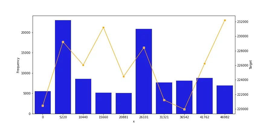
Figure 5: A graph for univariate analysis that shows a weak correlation
Bivariate Analysis
Bivariate Analysis comprises of finding co-relation between different features and selecting the features that are unique. If two features are highly correlated, we need to get rid of one of them, as a redundant presence introduces bias in the algorithm.
Towards this effort, we often create a heatmap using Pearson or Spearman correlation. The following figure shows how a heatmap represents the correlation coefficient. We set a threshold for the features, and if any two features are more corelated than the decided upon threshold, we either remove one of the two or combine them using Principal Component Analysis.
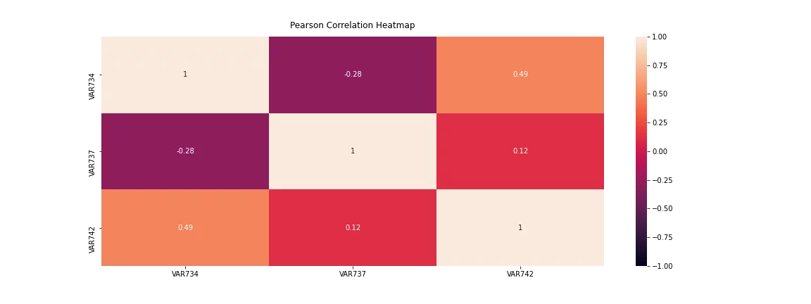
Figure 6: A heatmap of bivariate analysis of selected features
Note: Principal component analysis is where we merge two features to create a new one. The detail of this technique is a whole another discussion, but we will briefly discuss them below.
Feature Transformation
Another part of feature engineering is feature transformation. Feature transformation is utilized when the default representation of a variable is not suitable for the algorithm or when the transformation can help in making more accurate predictions. A few common feature transformations are discussed below:
Feature Scaling
Feature scaling is one of the most important steps in data pre-processing. A dataset may have several variables, each with its own range of values. This difference can introduce a bias in the machine learning algorithm. A value with a higher range can take precedence over the one that is lower.
In addition to this, non-scaled data hinders the gradient descent procedure and leads to a slower convergence. By bringing the data to a comparable or same scale, both issues can get resolved. The following diagram efficiently explains how the gradient descent may vary in scaled and non-scaled data.
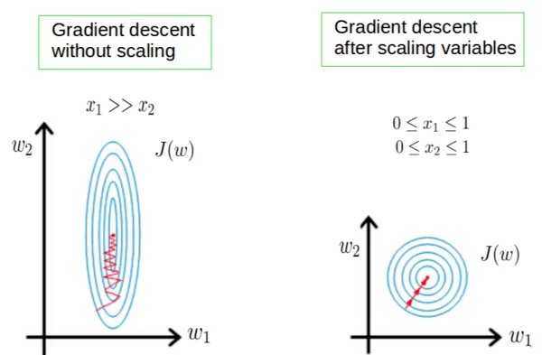
Figure 7: Effects of Scaling on gradient descent.
Feature Normalization
Sometimes the values in a continuous feature are highly skewed. This makes it difficult for the values to be compared and reduces the capability of the machine learning algorithm to extract a pattern. In such cases, we use statistical transformations. Log Transformation is quite popular and serves the purpose quite well.
The ‘Log transformation’ takes an instance ‘x’ of the data and replaces it with ‘log(x).’ This transforms the data into a much more suitable range and introduces normal distribution in the data. But there is a limitation to this method. Log transformation works effectively – to transform the data into normal distribution – only when the original data closely follows logarithmic distribution i.e., it is positively skewed.
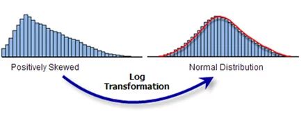
Figure 8: Effect of Log Transformation
An ‘Exponential transformation’ can have a similar effect of converting the data to normal distribution if the original data is negatively skewed.
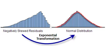
Figure 9: Effect of exponential Transformation
One Hot Encoding
Another data type that is incompatible is a categorical feature in non-numerical value, because most machine learning algorithms do not accept non-numerical values. Even if the value is in numerical type, if left untreated, the machine learning algorithm will consider the magnitude of the value as significant information. This often is not the case with categorical variables as they are present to distinguish between several types. For that, we convert them as follows.
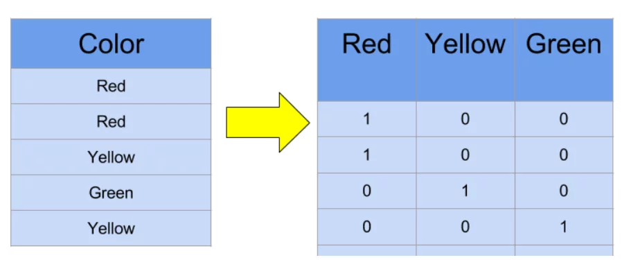
Figure 10: One Hot Encoding of a categorical variable creating new binary variables.
Here, instead of a single color-column we introduce a separate column for each unique categorical value. The values in these will be strictly binary and only one of them will be ‘1’ while all others will be ‘0’, based on original categorical value.
Explore Advanced Feature Engineering Techniques
Principal Component Analysis
Principal component analysis is a statistical feature crafting technique and is used to create a new feature that is representation of others. It has been widely used in fields such as computer vision and with the advent of bigdata, it has become popular in more mainstream data analysis problems.
PCA allows us to take several features with missing data, imprecisions, and other fallacies to merge them into one to get the most information out and stored in them. Mathematically, PCA tries to find a regression line in a k-dimensional plane that fits the k feature point the best with the least variance. This line is the new feature that can potentially replace the feature that PCA is performed upon.

Figure 11: Principal component Analysis performed over X1, X2 and X3 forms a projection line with minimal residual variance.
Conclusion
The field of data analysis runs quite deep and any of the topics mentioned briefly in this blog have material worth of a full blog on its own. There is a plethora of techniques, out of which only a few were mentioned here, each with its own quirks, that can be used in different cases. One thing that I must mention is that this is an iterative procedure, and each iteration will bring more insight into the problem. So, keep experimenting and keep improving.
Stay tuned for a technical guide of these methodologies.